Custom charts are visualizations you create explicitly. Use custom charts to visualize complex data relationships and have greater control over the appearance and behavior of the chart.

To create a custom chart, you can either:

• Build a chart in the W&B App by pulling in data from your runs using a GraphQL query.
• Log a wandb.Table and call the wandb.plot() function from your script.

import wandb
import math

with wandb.init() as run:
  offset = random.random()
  for run_step in range(20):
    run.log({
        "acc": math.log(1 + random.random() + run_step) + offset,
        "val_acc": math.log(1 + random.random() + run_step) + offset * random.random(),
    })

Create a custom chart in the W&B App

To create a custom chart in the W&B App, you must first log data to one or more runs. This data can come from key-value pairs logged with wandb.Run.log(), or more complex data structures like wandb.Table. Once you log data, you can create a custom chart by pulling in the data using a GraphQL query.

Suppose you want to create a line plot that shows the accuracy as a function of training step. To do this, you first log accuracy values to a run using the following code snippet:

import wandb
import math

with wandb.init() as run:
  offset = random.random()
  for run_step in range(20):
    run.log({
        "acc": math.log(1 + random.random() + run_step) + offset,
        "val_acc": math.log(1 + random.random() + run_step) + offset * random.random(),
    })

Each call to wandb.Run.log() creates a new entry in the run’s history. The step value is automatically tracked by W&B and increments with each log call.

Once the code snippet completes, navigate to your project’s workspace:

1. Click the Add panels button in the top right corner, then select Custom chart.
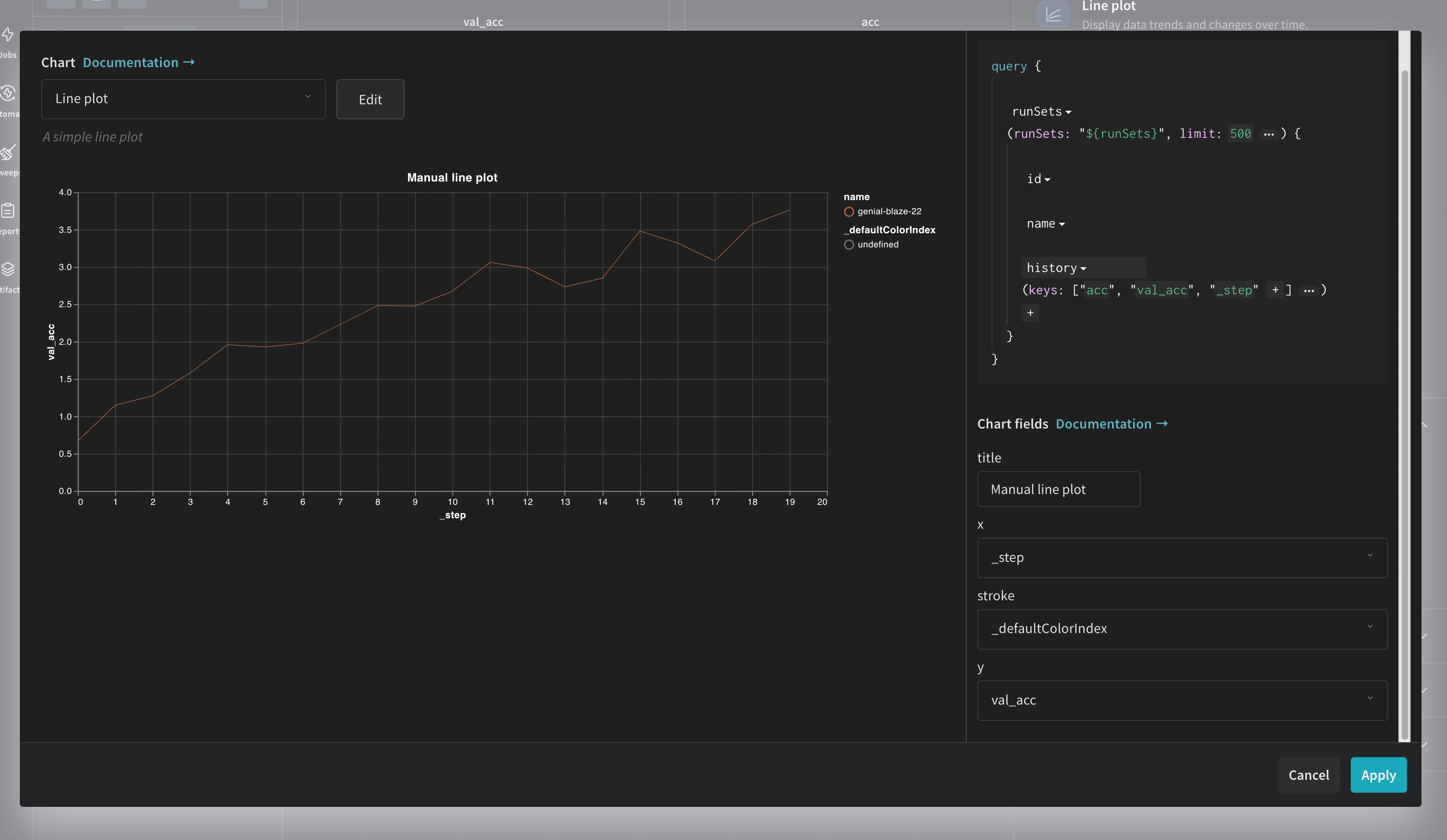
2. Select Line plot from the list of chart types.
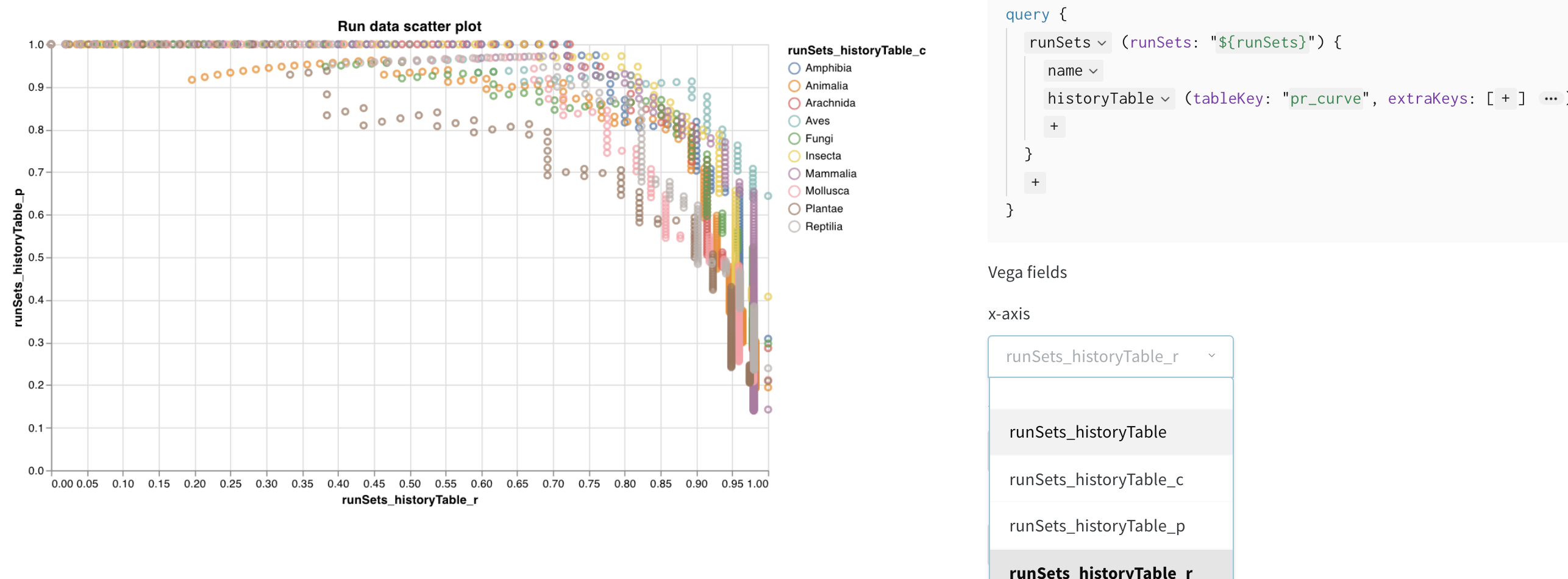
3. Within the query editor, select history as the data source. Next, select acc and type in _step as keys.
4. Within the chart editor, select _step for the X field and acc for the Y field. Optionally, set a title for the chart. Your settings should look similar to the following: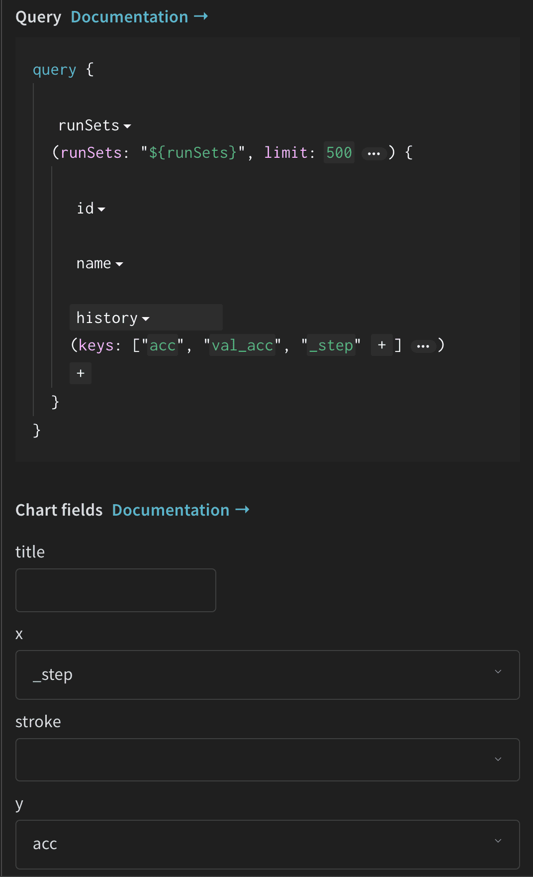

Your custom line plot should now appear in the panel, showing the accuracy values over training steps.

Query data sources

When you create a custom chart, you can pull in data from your runs using a GraphQL query. The data you can query comes from:

• config: Initial settings of your experiment (your independent variables). This includes any named fields you’ve logged as keys to wandb.Run.config at the start of your training. For example: wandb.Run.config.learning_rate = 0.0001
• summary: A single-value metrics that summarize a run. It’s populated by the final value of metrics logged with wandb.Run.log() or by directly updating the run.summary object. Think of it as a key-value store for your run’s final results.
• history: Time series data logged with wandb.Run.log(). Each call to log() creates a new row in the history table. This is ideal for tracking metrics that change over time, like training and validation loss.
• summaryTable: A table of summary metrics. It’s populated by logging a wandb.Table to the summary field. This is useful for logging metrics that are best represented in a tabular format, like confusion matrices or classification reports.
• historyTable: A table of time series data. It’s populated by logging a wandb.Table to the history field. This is useful for logging complex metrics that change over time, like per-epoch evaluation metrics.

To recap, summary and history are the general locations for your run data, while summaryTable and historyTable are the specific query types needed to access tabular data stored in those respective locations.

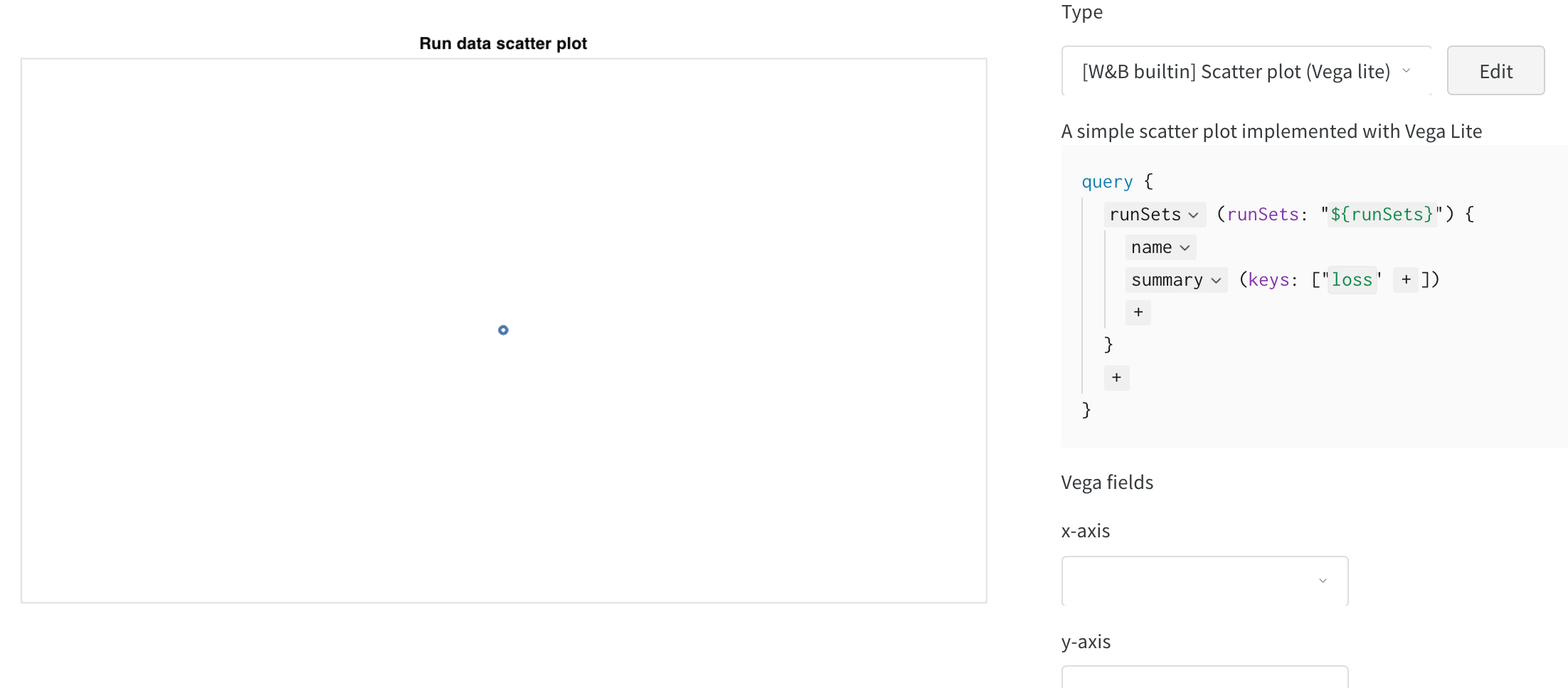
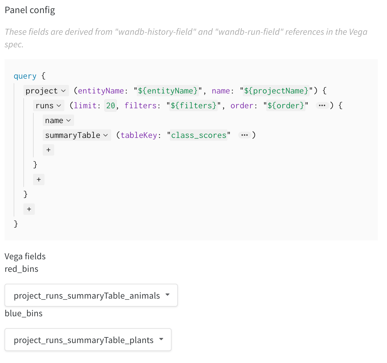
Query editor

Within the query editor, you can define a GraphQL query to pull in the data from available data sources. The query editor consists of dropdowns and text fields that allow you to construct the query without needing to write raw GraphQL. You can include any combination of available data sources, depending on the data you want to visualize.

The keys argument acts as a filter to specify exactly which pieces of data you want to retrieve from a larger data object such as summary. The sub-fields are dictionary-like or key-value pairs.

The general structure of the query is as follows:

query {
    runSets: (runSets: "${runSets}", limit: 500 ) {
        id: 
        name: 
        summary:
            (keys: [""])
        history:
            (keys: [""])
        summaryTable:
            (keys: [""])
        historyTable:
            (keys: [""])
    }
}

Here’s a breakdown of the components:

• runSets: Top-level object, representing the set of runs you are currently viewing or have filtered in the UI.
• summary(...), history(...), summaryTable(...), historyTable(...): This tells the query to fetch data from the respective objects of each run.
• keys: [""]: An array of strings where each string is the name (or key) of the metric or object you want to retrieve.

Log charts from a script

You can programmatically create a custom chart from your script by logging a wandb.Table of the data you want to visualize, then calling wandb.plot.* to create the chart.

For example, consider the following code snippet:

import wandb
import math

with wandb.init() as run:
    offset = random.random()

    # Set up data to log in custom charts
    data = []
    for i in range(100):
    data.append([i, random.random() + math.log(1 + i) + offset + random.random()])

    # Create a table with the columns to plot
    table = wandb.Table(data=data, columns=["step", "height"])

    # Use the table to populate various custom charts
    line_plot = wandb.plot.line(table, x='step', y='height', title='Line Plot')
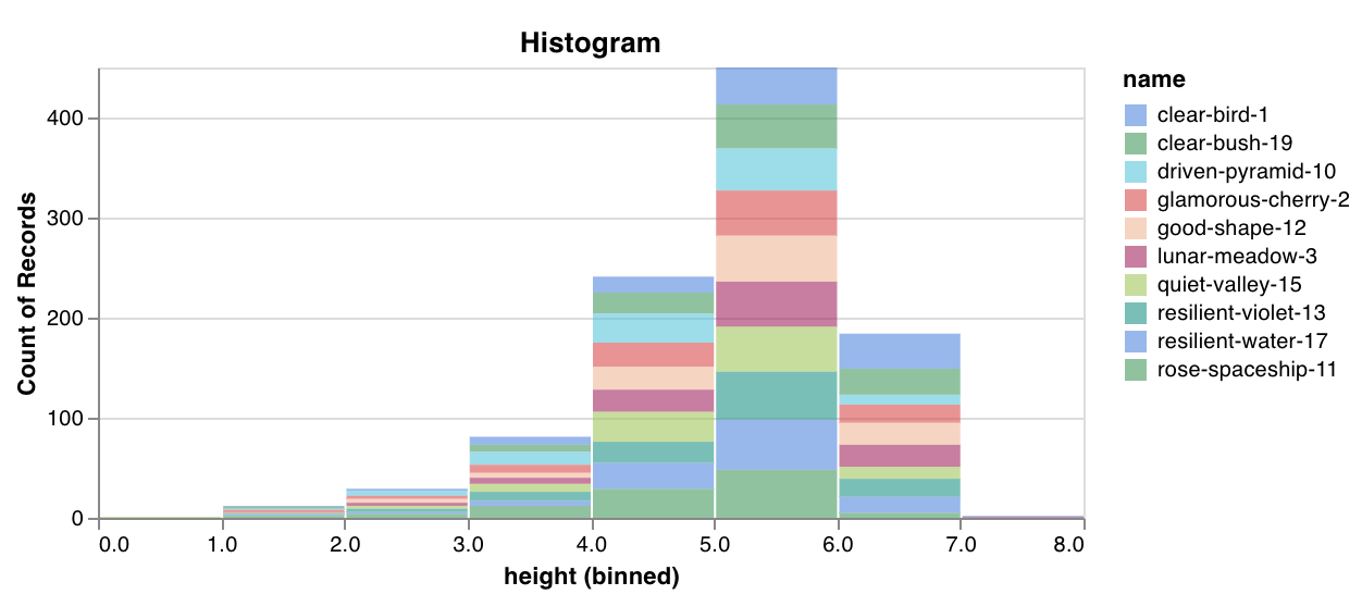
    histogram = wandb.plot.histogram(table, value='height', title='Histogram')
    scatter = wandb.plot.scatter(table, x='step', y='height', title='Scatter Plot')

    # Log custom tables, which will show up in customizable charts in the UI
    run.log({'line_1': line_plot, 
                'histogram_1': histogram, 
                'scatter_1': scatter})

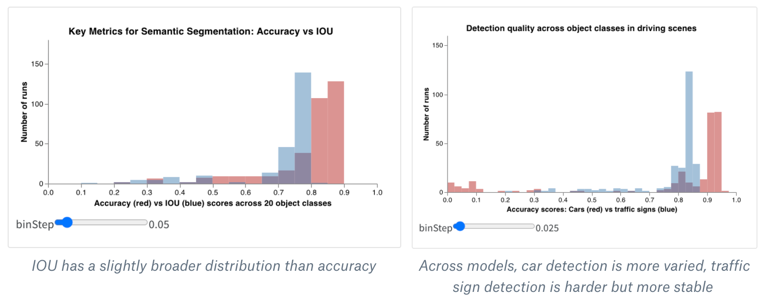
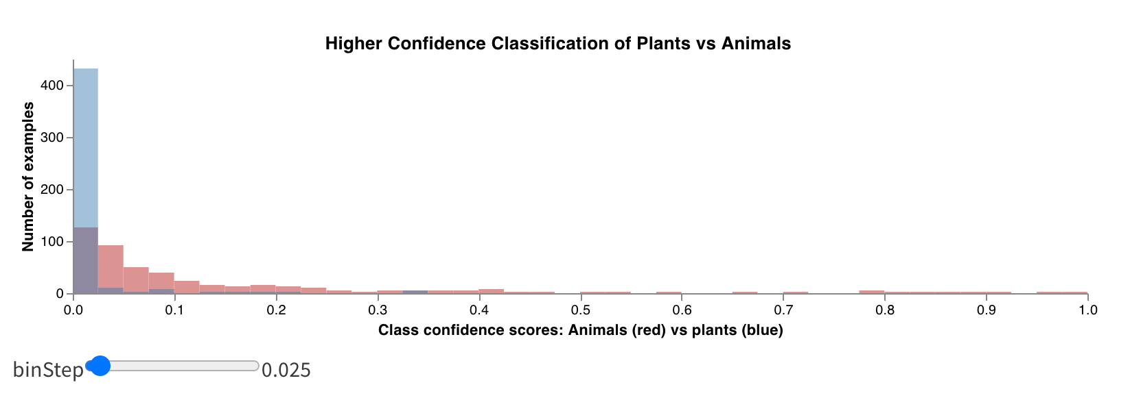
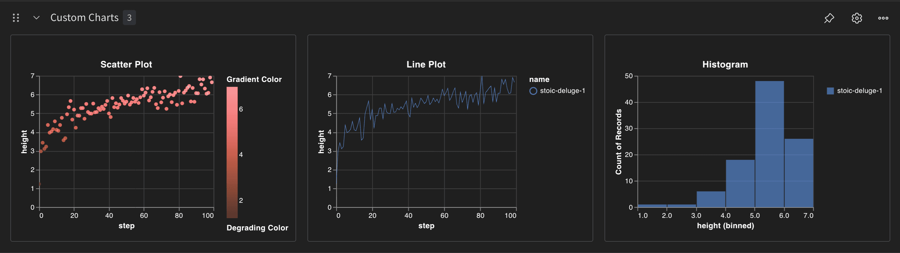
Within the W&B app, navigate to the Workspace tab. Within the Custom Charts panel, there are three charts with the following titles: Scatter Plot, Histogram, and Line Plot. These correspond to the three charts created in the script above. The x-axis and y-axis are set to the columns specified in the wandb.plot.* function calls (height and step).

The following image shows the three custom charts created from the script:

Built-in chart types

W&B has a number of built-in chart presets that you can log directly from your script. These include line plots, scatter plots, bar charts, histograms, PR curves, and ROC curves. The following tabs show how to log each type of chart.

• Line plot
• Scatter plot
• Bar chart
• Histogram
• PR curve
• ROC curve

wandb.plot.line()

Log a custom line plot—a list of connected and ordered points (x,y) on arbitrary axes x and y.

with wandb.init() as run:
  data = [[x, y] for (x, y) in zip(x_values, y_values)]
  table = wandb.Table(data=data, columns=["x", "y"])
  run.log(
      {
          "my_custom_plot_id": wandb.plot.line(
              table, "x", "y", title="Custom Y vs X Line Plot"
          )
      }
  )

A line plot logs curves on any two dimensions. If you plot two lists of values against each other, the number of values in the lists must match exactly (for example, each point must have an x and a y).

See an example report or try an example Google Colab notebook.

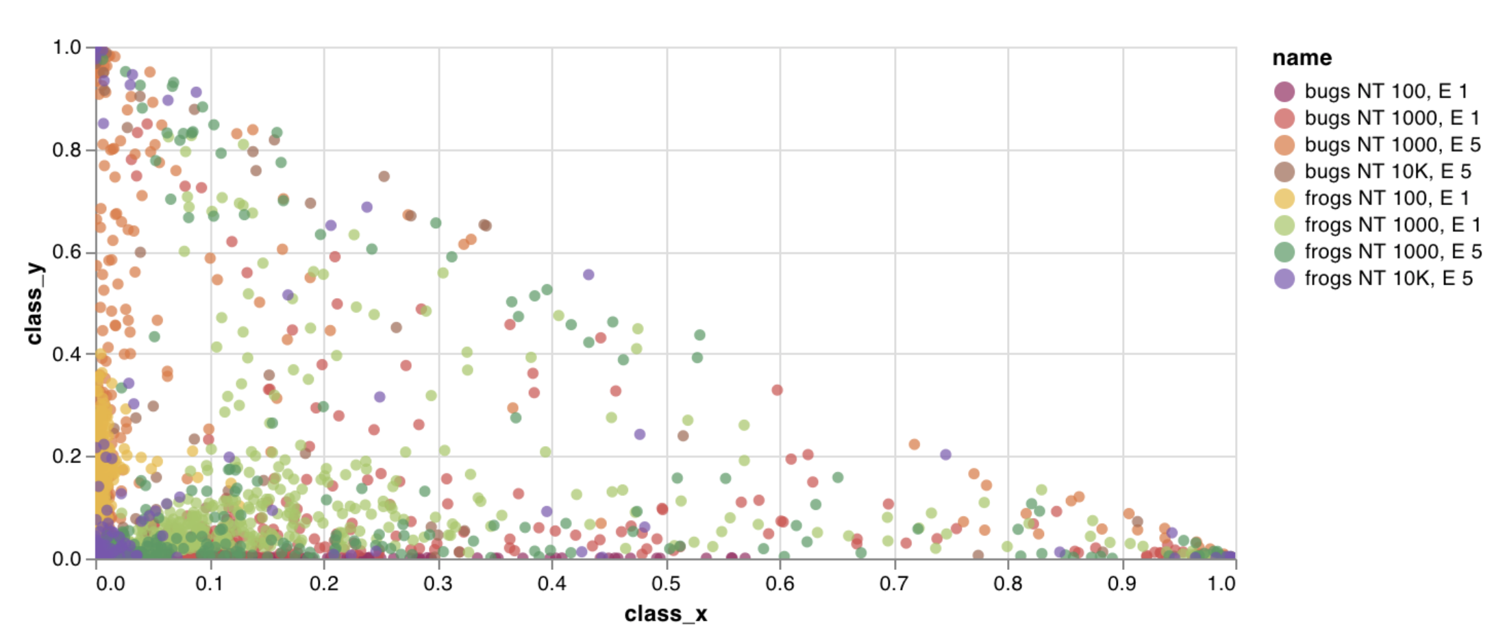
wandb.plot.scatter()

Log a custom scatter plot—a list of points (x, y) on a pair of arbitrary axes x and y.

with wandb.init() as run:
  data = [[x, y] for (x, y) in zip(class_x_prediction_scores, class_y_prediction_scores)]
  table = wandb.Table(data=data, columns=["class_x", "class_y"])
  run.log({"my_custom_id": wandb.plot.scatter(table, "class_x", "class_y")})

You can use this to log scatter points on any two dimensions. Note that if you’re plotting two lists of values against each other, the number of values in the lists must match exactly (for example, each point must have an x and a y).

See an example report or try an example Google Colab notebook.

wandb.plot.bar()

Log a custom bar chart—a list of labeled values as bars—natively in a few lines:

with wandb.init() as run:
  data = [[label, val] for (label, val) in zip(labels, values)]
  table = wandb.Table(data=data, columns=["label", "value"])
  run.log(
      {
          "my_bar_chart_id": wandb.plot.bar(
              table, "label", "value", title="Custom Bar Chart"
          )
      }
  )

You can use this to log arbitrary bar charts. Note that the number of labels and values in the lists must match exactly (for example, each data point must have both).

See an example report or try an example Google Colab notebook.

wandb.plot.histogram()

Log a custom histogram—sort list of values into bins by count/frequency of occurrence—natively in a few lines. Let’s say I have a list of prediction confidence scores (scores) and want to visualize their distribution:

with wandb.init() as run:
  data = [[s] for s in scores]
  table = wandb.Table(data=data, columns=["scores"])
  run.log({"my_histogram": wandb.plot.histogram(table, "scores", title=None)})

You can use this to log arbitrary histograms. Note that data is a list of lists, intended to support a 2D array of rows and columns.

See an example report or try an example Google Colab notebook.

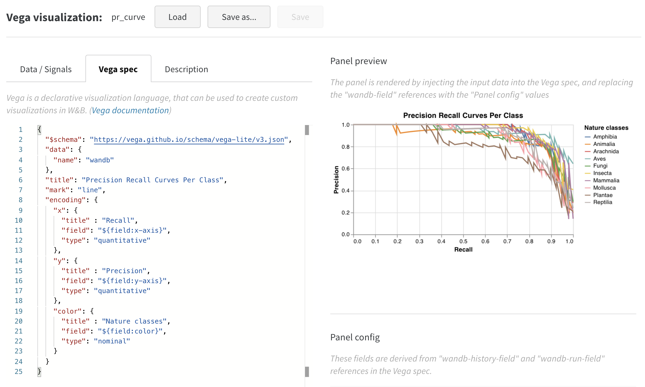
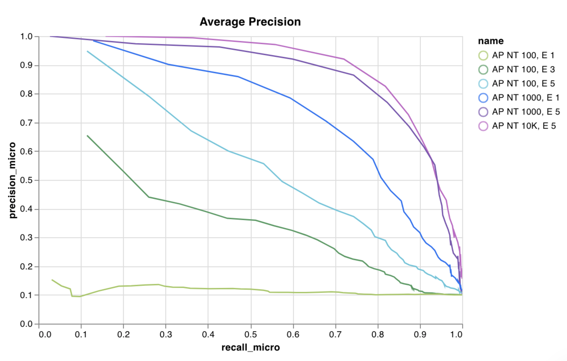
wandb.plot.pr_curve()

Create a Precision-Recall curve in one line:

with wandb.init() as run:
  plot = wandb.plot.pr_curve(ground_truth, predictions, labels=None, classes_to_plot=None)

  run.log({"pr": plot})

You can log this whenever your code has access to:

• a model’s predicted scores (predictions) on a set of examples
• the corresponding ground truth labels (ground_truth) for those examples
• (optionally) a list of the labels/class names (labels=["cat", "dog", "bird"...] if label index 0 means cat, 1 = dog, 2 = bird, etc.)
• (optionally) a subset (still in list format) of the labels to visualize in the plot

See an example report or try an example Google Colab notebook.

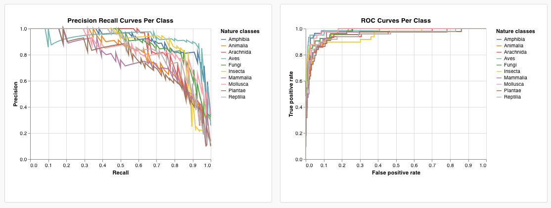
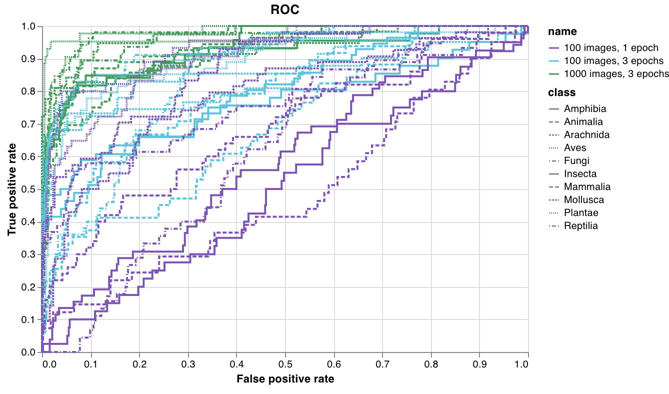
wandb.plot.roc_curve()

Create an ROC curve in one line:

with wandb.init() as run:
  # ground_truth is a list of true labels, predictions is a list of predicted scores
  ground_truth = [0, 1, 0, 1, 0, 1]
  predictions = [0.1, 0.4, 0.35, 0.8, 0.7, 0.9]

  # Create the ROC curve plot
  # labels is an optional list of class names, classes_to_plot is an optional subset of those labels to visualize
  plot = wandb.plot.roc_curve(
      ground_truth, predictions, labels=None, classes_to_plot=None
  )

  run.log({"roc": plot})

You can log this whenever your code has access to:

• a model’s predicted scores (predictions) on a set of examples
• the corresponding ground truth labels (ground_truth) for those examples
• (optionally) a list of the labels/ class names (labels=["cat", "dog", "bird"...] if label index 0 means cat, 1 = dog, 2 = bird, etc.)
• (optionally) a subset (still in list format) of these labels to visualize on the plot

See an example report or try an example Google Colab notebook.

Additional resources

• Log your first custom chart with this Colab notebook or read its companion W&B Machine Learning Visualization IDE report.
• Try the Logging custom visualizations with W&B using Keras and Sklearn Colab notebook.
• Read the Visualizing NLP Attention Based Models report.
• Explore the Visualizing The Effect of Attention on Gradient Flow report.
• Read the Logging arbitrary curves report.